Statistics Views

Statistics views are visually enhanced representations of specific requests especially tailored for optimal performances allowing powerful interactive manipulation. They are indispensable tools aimed at being used in conjunction with all others graphical views in order to progress meaningfully through the investigation.

Common features

All the statistics views have a lot of features in common. In fact, the main distinction between them is pretty much a matter of interpretation…

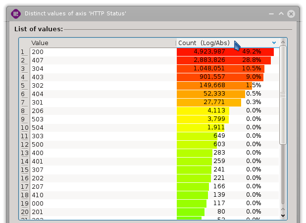
Frequency representation

The list of values can be sorted alphabetically or by frequency by clicking on the horizontal header of the desired column.

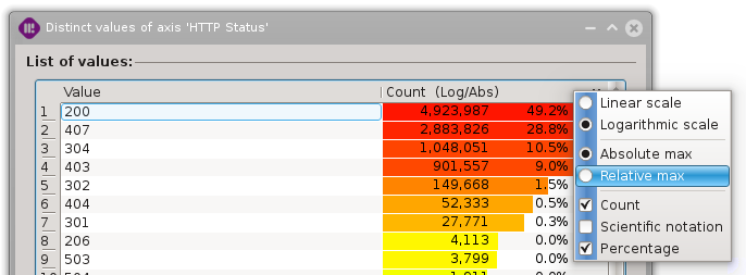
Frequency representation can be customized by right-clicking on the horizontal header of the desired column.

1. Scale can be toggled between: * Linear * Logarithmic

2. Maximum reference count can be toggled between: * Absolute : Percentage relative to the total of selected lines (also set scale to “Logarithmic”) * Relative : Percentage relative to the number of occurences of the most represented value (also set scale to “Linear”)

3. Frequency can be expressed by a combination of the following informations: * Occurence count * Scientific notation * Percentage

Selecting values

Values can be selected using three different approaches:

1. Using specific values (Ctrl+Click)

2. Using a range of specific values (Shift+Click)

3. Using a specific frequency range (Frequency widget).

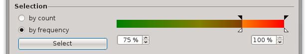
The lower and upper bounds of the frequency widget can be defined by left-clicking or right-clicking in the color-ramp. They can then be dragged to refine their position. At last, the checkboxes can also be used to achieve the maximal precision, especially when using the count mode.

Note

Sliders are positionned on the color gradient according to the selected scale to provide smoother selections.

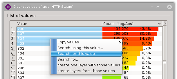
Actions can then be made on the selected values, like applying search filters or exporting values using the contextual menu on selected values.

Layer creation

New layers can be created from the context menu of statistics views using the selected values; two creation modes are available:

• one layer containing all the selected values

• one layer for each selected value

A dialog permit to parametrize the layer creation.

New layers’ naming

A free string with three substitution patterns:

• %l for the name of the current layer

• %a for the name of the observed axis

• %v for the selected values list

Where the new layers will be inserted in the layer stack

• at the of top of it (this is the default)

• above the current Layer

• below the current Layer

Exporting values

See Exporting statistics

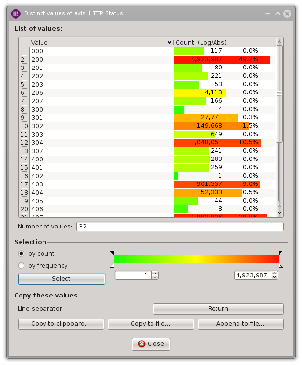
Distinct values dialog

This statistics view provides a list of distinct values with their frequencies for any given column of the listing view.

Note

This is equivalent to the SQL query ‘SELECT column, COUNT(*) FROM current_selection GROUP BY column’.

Accessing the dialogs

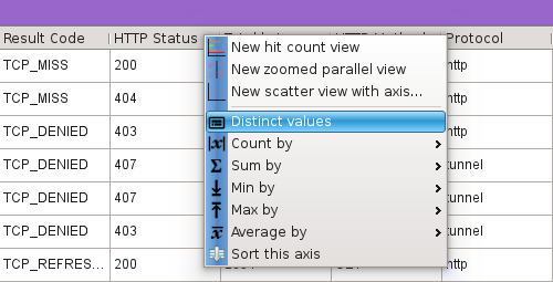
There are two ways to access these dialogs.

By right-clicking of the horizontal header of the desired column in the listing view,

or by clicking on the icon on the statistic panel located in the bottom of the listing view.

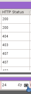
Clicking on the refresh icon will display the number of distinct values in the panel.

Count by dialog

The count by dialog allows to count the number of distinct values on a secondary axis for each distrinct value on a given axis.

Note

This is equivalent to the SQL query ‘SELECT column1, COUNT(DISTINCT column2) FROM current_selection GROUP BY column1’.

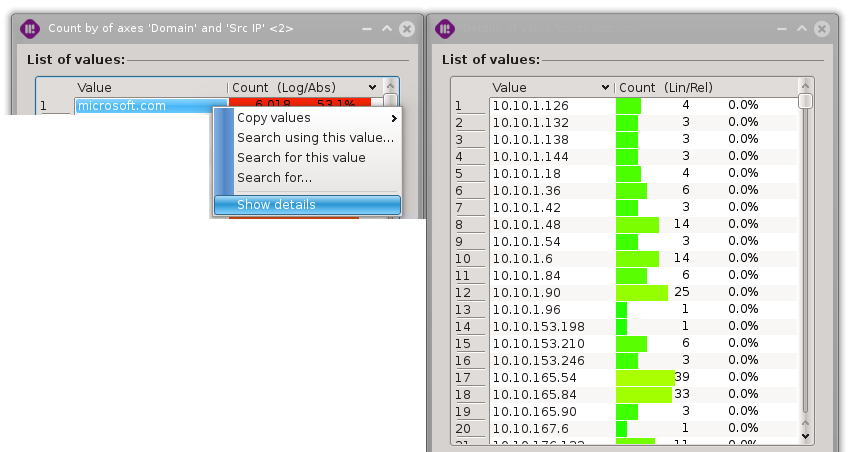
As an example, we wish to count the values of the ‘Domain’ axis by the values of the ‘Src IP’ axis in order to figure out which domains are the most widely accessed.

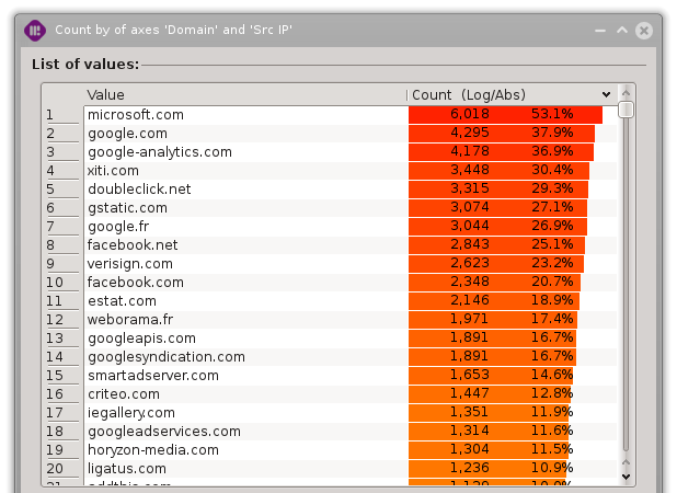
In our case, ‘microsoft.com’ is classed 1^st^ with a frequency of 53.1% because a bit more of half the source IP has reached microsoft.com. As the frequency is based on the distinct values count of the secondary axis, the sum of all the frequencies is unlikely to be 100% as for the distinct values dialog.

For each value of the primary axis, the list of the distinct values present on the secondary axis can be shown by right clicking on a value and selecting “Show details”.

For information, here are the distinct values counts of the previously used axes:

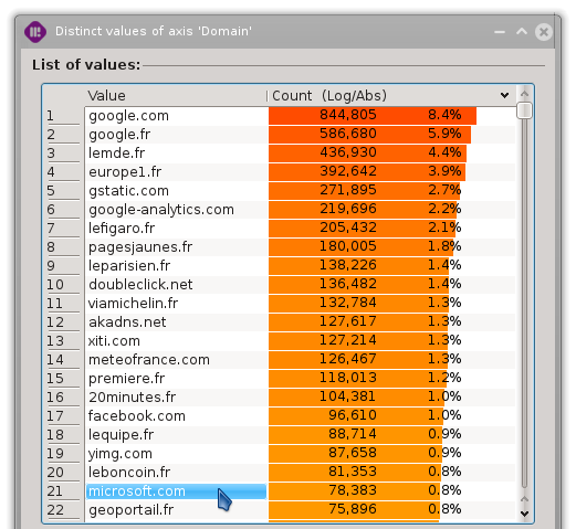
“Domain” distinct values

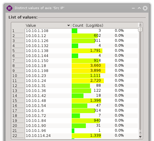
“Src IP” distinct values

As we can see, ‘microsoft.com’ is only in the 21^th^ position when its frequency is based on the total amount of events.

Sum by dialog

The sum by dialog allows to sum the values on a secondary axis for each distinct value on a selected axis.

Note

This is equivalent to the SQL query ‘SELECT column1, SUM(column2) FROM current_selection GROUP BY column1’.

As an example, we wish to sum the ‘Total bytes’ fields of the ‘Src IP’ column in order to get an ordering of the bandwidth used by machines.

“Domain” distinct values

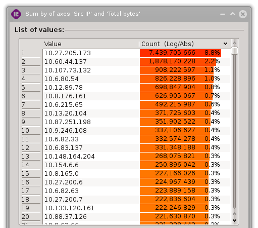
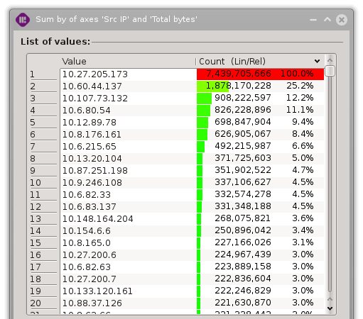
As we can see, one machine is consuming 8.8% of the total bandwidth (6.9GB). As a comparison, the second machine consuming the most bandwidth is only using 25.2% of the top one.

Min by dialog

The min by dialog allows to get the minimal values on a secondary axis for each distinct value on a selected axis.

Note

This is equivalent to the SQL query ‘SELECT column1, MIN(column2) FROM current_selection GROUP BY column1’.

Max by dialog

The max by dialog allows to get the maximal values on a secondary axis for each distinct value on a selected axis.

Note

This is equivalent to the SQL query ‘SELECT column1, MAX(column2) FROM current_selection GROUP BY column1’.

Average by dialog

The max by dialog allows to get the average values on a secondary axis for each distinct value on a selected axis.

Note

This is equivalent to the SQL query ‘SELECT column1, AVG(column2) FROM current_selection GROUP BY column1’.